Stratigraphic pick prediction via supervised machine-learning: Predictatops

Presentation of Predictatops

Back in May, I presented a talk at the 2019 AAPG ACE (American Association of Petroleum Geologist Annual Conference and Exhibit) on using machine-learning to predict stratigraphic surfaces in well logs. I described a Python projects I have been working on as a side project called Predictatops. Given I’ve mentioned working on the issue of stratigraphic top prediction using machine-learning in previous blog posts, I thought it wise to announce Predictatops here on my website as well.

Predictatops Logo

Definitions

First, some definitions for the machine-learning folks who stumbled into a geologist blog post and the geologists who stumbled into a machine-learning blog post…

Wells:

Holes drilled in the ground.

Well Logs:

Well logs are created when a geophysical measurements are made along a well. These are usually 1D measurements in the sense that a measurement is made at the bottom, then the tool is pulled up a little bit and then another measurement is made. This continues until the entirety of the well is measured. Often, many different types of tools are used that measure different properties, resulting in multiple well logs for a single well. They measure things like how fast sound travels between two parts of the well or how much signal is bounced back and measured by a tool after a certain type of radiation is given off by a tool. These measurements are then turned into rock properties like density, grain size, etc. Further explanations of well log measurements are here and here. The picture below is of a well log.

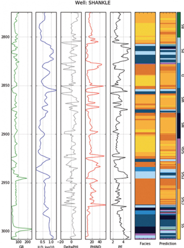Well logs from a single well. Interpretation of lithology of the rocks on the right in colored bars. Hall at al., 2015

Tops:

Tops are markers for the tops of things. Specifically, tops of geologic units. Everything below a top is one geologic layer and everything above a top is another geology layer.

Different Types of Tops:

Tops can divide different categories of layers. Sometimes the layers are based on characteristics of the rock. For example a top can separate rock made from small grains from rock made of large grains. Tops based on physical make-up of rocks are often called lithologic tops. Lithology is term for describing what a rock is made up of. Facies is another term that refers to categories of rocks in a well with similar characteristics.

Alternatively, tops can be boundaries based on more actionable characteristics like the ability for fluids to flow. A top might separate a geologic layer where you think the rock will allow fast flow of fluids like water, oil, or gas from a layer below the top where fluids will flow very slowly.

Geologists' favorite way to place a top, however, is to place tops based on time. A top can separate rock deposited at one point in time from rock deposited at the next point of time. This is a stratigraphic or chronostratigraphic top! Also, called a time surface.

You might have noticed that the lithologic, flow-based, and stratigraphic tops are increasingly abstract.

The first, lithologic-tops are based on what the rock is made up of, which can be measured, at least indirectly. Flow is a little harder to predict from well logs but the ability of fluids to flow is fundamentally also based on physical characteristics, which can be measured, just with more difficulty as very small characteristics at the level of pores in rocks are what matter.

Stratigraphic tops are based on age of the rocks. There is no measurement that relates to time that can be done routinely in well logs. You can collect fossils and interpret time based on the fossils found in different units (biostratigraphy). You can find volcanic ash and date it by looking at how much one type of element has turned into a different type of element due to decay (geochronology). However, neither of these can be done on all, or even most, wells. They’re too expensive and time consuming. Not all depth points will have fossils or ash layers for dating.

Stratigraphic Correlation:

How then does one go from well logs to stratigraphic tops representing time surfaces? That requires a model, and a head to put it in.

In practice, chronostratigraphic (mapping out time surfaces) well log correlation (correlation means interpreting where a top in well A exists in well B) is a combination of lithostratigraphic correlation (looking at 2 wells and matching curves of the well logs using the assumption that similar looking curves, have similar properties, and are the same layers) and application of conceptual models. These conceptual models cover how sediment is transported and deposited. They are very helpful for stratigraphic correlations as they predict the spatial distribution of different types rocks deposited at the same time and how those spatial associations can change over time. These conceptual models come from two places, outcrop studies (going out in the field and looking at rocks) and modern analogues studies (going out to the valley, rivers, lakes, oceans, etc. and seeing how sediment gets deposited). The geology name for these conceptual models is depositional environments. Some additional information on them can be found here. Another key conceptual model is sequence stratigraphy.

An example of lithostratigraphic vs. chronostratigraphic interpretation below.

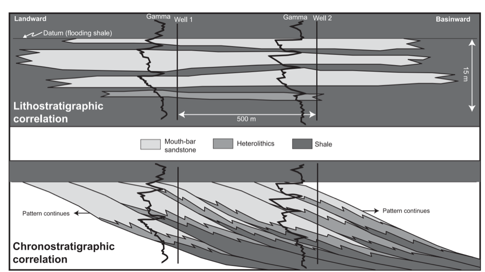The top picture shows lithostratigraph correlation where the assumption is that rocks with similar characteristics are deposited at the same time. The bottom is a chronostratigraphic interpretation where models from outcrop studies of deltas are used as a guide. In the deltaic depositional environment, the coarser grains are deposited first and then finer grains, which build up over time as sheets angled towards the deeper water. The lower interpretation is correct.

You can read more about stratigraphic well log correlation from this page by SEPM (a national sedimentology association).

Just to be clear, with Predictatops, we are wanting to do chronostratigraphic correlation, not lithostratigraphic correlation.

Supervised Machine-learning:

In our context, supervised machine-learning means, instead of letting the computer going on fun field trips like geologists to gradually build up mental conceptual models to use for correlating well logs chronostratigraphically, we’ll give the computer a dataset of already human-picked tops for one time surface and ask the computer to figure out a model that lets it mimic the geologist.

For more detailed explanations of machine-learning, there are lots of things on the web that google will provide for you. I’m a fan of the medium articles by “Cassie Kozyrkov” whose title is “Chief Decision Intelligence Engineer, Google” and does a good job at packaging key points in an entirely dense but fun to read space.

Building Geologic Observations into Features:

Features in a machine-learning context are new data characteristics built from the original data. An basic example might be the sum of three other original data characteristics. Feature creation is a very common part of machine-learning. Rarely would you only use original raw data.

Unlike some of the demo datasets traditionally used in machine-learning demos where each row of the dataset is an independent entity and features are only created within each row, a key aspect of building features for stratigraphy applications is that a lot of valuable information can be gleaned if one creates features based on comparisons or aggregate observations from multiple depth points or even across wells. One type of comparison is between each depth point in question and the depth points above, below, and around it within different length windows. Another type of comparison is between the characteristics of the well that holds the depth point being predicted for and the neighboring wells.

These comparison-based features are similar to what a geologist does visually when they put wells in a cross-section, or a sequence of wells’ well logs, and attempt to pick where stratigraphic tops should be correlated as shown below.

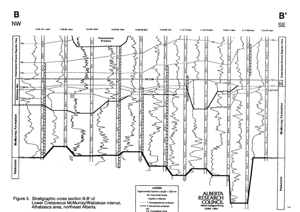A cross-section showing different tops in different wells. Vertical curvy lines are gamma-ray well log curves. Alberta Geological Survey Open File Report 1994-14. Cross-section B to B'.

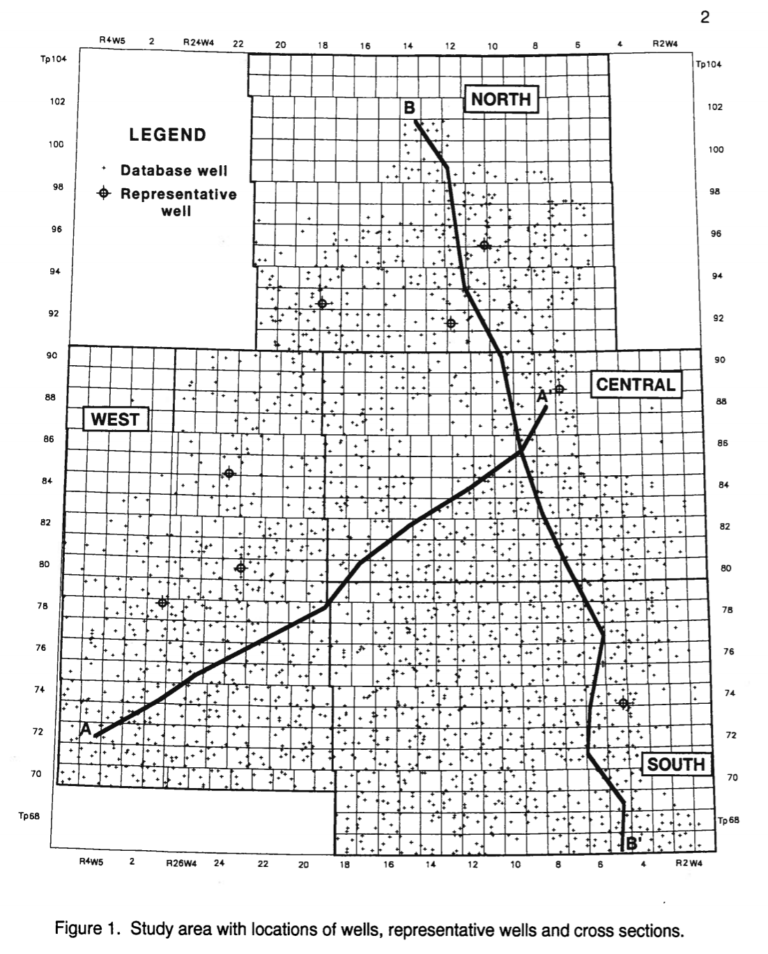Map of Mannville wells in the Alberta Geological Survey open file report 1994-14 that are used in the project I’m doing at the github link.

Only creating features based on data in individual depth points in individual wells would like cutting up all your well logs from all your wells into little bits, giving them to your geologist in a bucket, shaking the bucket, and then ask the geologist which depth point pieces are the same depth as the top you’re trying to predict for. Obviously, that wouldn’t work out so well. If you were to set up a stratigraphic machine-learning project and only create features from data at the same depth points for each well, you’d be doing the same thing to your machine-learning model.

Predictatops: Supervised Machine-Learning of Stratigraphic Surfaces

Predictatops Supervised Machine-learning Goal:

The goal of Predictatops is to be able to give it a training datasets of wells (that include both well logs and trusted human-assigned tops) for a single time surface and a test datasets of just well logs and get back where it thinks the top should be in each well in the test dataset.

How to judge success:

We want to minimize the distance between where the ML model predicted the top should be in each well and where the human(s) put the top. That difference will be our error. For comparing different runs we’ll return the RMSE (root mean squared error) for the top we’re trying to predict across all the wells.

We could have picked a different way to judge prediction success, so I’ll explain a bit about why I think this is a better way.

You might be tempted to set the problem up as a classification problem where we don’t predict a single pick but rather for each depth point in every well predict what formation (another geology word for layer) that depth point is. The problem with doing it this way, is that geologist really don’t care whether you got the formation correct far away from any top. That might not even be a hard problem. Additionally, how good your statistics appear to be will be affected by how thick the layers are, which isn’t ideal.

You could also frame the problem in terms of a binary question of whether or not the top was predicted to be in the exact same place as the geologist put it. The problem with this approach is two-fold. First, you immediately have a huge imbalanced class problem on your hands. If your well logs have a different measurement every 1/3 of a meter and typically are 300 meters long, every well will have 1 instance of data to represent the top and 899 instances to represent not the top. This will make machine-learning very difficult. Second, a binary prediction approach will affect the way you judge accuracy resulting in some not particularly useful information. You might get 4% of the depths predicted exactly right and 96% wrong. However, if all your 96% wrong tops are within plus or minus 2 meters of the actual tops, that’s amazing good. If the average distance between the actual top and predicted top is plus or minus 56 meters, that’s not good. In both cases, you were only 4% accurate.

Project setup:

If we can’t set-up the problem as a binary machine-learning program or a classification machine-learning problem, how do we set up the problem?

In Predictatops, we handled this by making it a two-step prediction with the first step being classification, not on formation labels, but on distance zones away from the pick we were trying to predict. Imaginary zones were created at the pick, slightly away from the pick below, slightly away from pick above, farther form pick below, farther from pick above, and everything else. We then ran classification to predict the zone of each depth point in each well. Those results were then run through an additional process that produced higher numbers for depth points that had the most predictions for being at the top or very near to the top around it. More of this process is described in this presentation given at AAPG ACE and in the documentation of Predictatops.

Data Requirements:

The supervised part of supervised machine-learning means you have to have human-labeled tops to start. In addition, you have to have enough wells from enough places that the full complexity of the stratigraphy is captured in the training wells. The exact number required is hard to define as it depends on the complexity of the problem, how generalizable we want to the solution, and the algorithms used. If you had to press me, I’ll say you’ll need several hundred tops, if not more than a thousand, for your training datasets.

While we’re discussing training dataset sizes, a point of interest here is that the number of required training wells goes down is someone is kinda enough to create and release open-source a pre-trained model on say 200,000+ wells in a depositional environment similar to yours. Then you might be able to use that model as a starting point and retrain it with your use-case specific training dataset. This is a over-simplistic description of transfer-learning, which has resulted in incredible gains in image and natural language processing machine-learning.

An additional data requirement is that these wells have the same, or at least very similar, well log types. Machine-learning likes all the inputs to be collected and prepped the same way. Although this may seem like a simple ask to those not in oil & gas, the reality is that many wells will be drilled with different well logs. Some types will be always present. Some types will be mostly present. Others rarely present. Some types, like sonic, will be very common but different tool vendors used that measure the same property in different ways. Well log normalization by petrophysicists may be required.

In the demo dataset from the McMurray formation, a collection of well logs that were in the highest number of wells were found. The impact of that constraint was that instead of 2000 wells used, just over 1200 wells were used. There are classes in Predictatops to help identify what well logs are the most common in a given dataset.

Predictatops Project Status:

Predictatops is functional but still changing. I tried to organize things such that large pieces could be skipped and others added without too much trouble. It has a demo data from the McMurray in Alberta, Canada and instructions for how to run it with that demo dataset. The documentation is still a work in process but the basics are all there. I’ve made some changes to make it more generalizable, but there is more to be done in that area.

Predictatops Performance:

The top McMurray currently has a RMSE (root mean squared error) of 6.6 meters. More information is available in this presentation given at AAPG ACE and in the documentation of Predictatops.

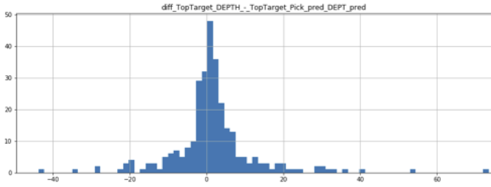A histogram showing the distribution of McMurray Top prediction error. Bars count how many wells where in each group. Groups are based on difference in depth between actual human-picked top and machine-picked top. RMSE is 6.6 m.

Wait, but I don’t trust my geologist.

Yes, one limitation of all of this is that fundamentally the machine-learning model is trying to mimic a person’s (or multiple people’s) top interpretations. The best you’ll get out of the machine-learning model in terms of performance accuracy is slightly worse than the training dataset supplied by human geologist(s).

When would you want to use this type of approach?

• When you don’t have enough time for a geologist to interpret all the wells, but you have enough time to interpret 1000 out of 7000 wells.
• When you have two areas worked by different geologists and you want to see how the interpretation of geologist A transfers to the neighboring area worked by geologist B.
• When you want to identify the 5% of the wells with the most uncertainty and have your best geologists focus on those.

Are there uses for this type of approach even if I already have human tops for all my wells?

Yes, the great thing about this type of approach is it scores each depth point in every well. That score can be normalized to a probability of how likely each depth point is to actually be the top. There are wells where only one depth point or a small cluster of depth points have higher scores. Other wells have high scores spread more widely throughout the well. Additionally, some wells have predicted tops at similar depths to their neighbors. Other wells do not. This information can be used to generate uncertainty scores/maps/curves and help geologists know where to focus their efforts. I haven’t done this with Predictatops yet, but it is totally possible!

Making it easy to use the demo dataset:

As mentioned before, the demo dataset comes from the McMurray formation in Alberta, Canada. There’s information on it in the README.md and documentation of Predictatops. The full reference is: Wynne et al., (1994) Athabasca Oil Sands Database McMurray/Wabiskaw Deposit, Open-File-Report 1994–14, Alberta, Canada; Alberta Geological Survey. Links to report & dataset. This is a great open-source dataset from the Alberta Energy Regulator and Alberta Geological Survey that could be used in a lot of other machine-learning focused work as it is one of the larger open-source datasets of a single formation already compiled and prepped by a single group.

Discovering, evaluating, loading, and transforming data takes a lot of time. There’s always a risk you’ll get through some or all of those steps and then discovery the dataset won’t work for your purposes. This dataset is already put together and can be used for both stratigraphic top prediction and facies prediction.

I’ve been working on a pull request for the Rockhound Python package, a project to make loading geologic demo datasets super quick and easy, that will let you pull in the fully prepped and merged McMurray dataset with two lines of code. Currently, there is this pull request for the McMurray dataset prepped for facies prediction. Once that pull request is accepted, I’ll push another dataset prepped for stratigraphic prediction.

Other Examples of Using Machine-Learning for Stratigraphy & Top Prediction

Lithostratigraphy:

Lithostratigraphy is basically curve matching, so computational approaches go back to the 1970s. Some of the better results seem to be geologic specific variations on dynamic time warping. One example is CORRELATOR from Kansas Geological Survey, but there are more modern approaches in Python as well.

The reasons for why this type of computational approach seemed to have never caught on are likely complex. I don’t claim to understand all of them, but I suspect it was related to the fact that they often didn’t return a single surface but rather an arbitrary number of surfaces. This meant the geologist still had to look at the well logs in order to use the results. Hence, the time savings aren’t there.

Chronostratigraphy:

If you’re interesting in this type of thing, here are two other recent examples of applying machine-learning to stratigraphy that I think are very interesting.

1. Alex Bayeh, Michael Ashby, Darrin Burton, and Seth Brazell at Anadarko (now Occidental) published “A Machine-Learning-Based Approach to Assistive Well-Log Correlation“, which uses thousands of pairs of well logs that are and are not representing the same layer to train a model, which is then used with a small number of tops from a specific formation and tops for that formation predicted. I was excited to see this type of approach because (1) I thought an approach sort of like this might be possible but don’t have access to large enough open-source dataset to actually attempt it myself (2) it demonstrates a different approach to supervised machine-learning applied to stratigraphy.
2. Additionally, there’s been a variety of papers trying to apply wavelet transform theory to well log correlation for the past two decades. My opinion of these approaches has typically been that there is a lot of complexity without that much to show for it in terms of useful predictions. A recent exemption to this was Ye at al., 2017‘s “Rapid and Consistent Identification of Stratigraphic Boundaries and Stacking Patterns in Well Logs – An Automated Process Utilizing Wavelet Transforms and Beta Distributions“, which looks like it would be an excellent feature creation step to use in supervised, or event unsupervised machine-learning, applied to stratigraphy.

Contributing to Predictatops

Pulls requests and issues (in the form of bugs, enhancements, comments, and even idle observations) are very welcome on Predictatops. I currently have 18+ issues on the repository for things to do. It is a side project, so please don’t expect it to be perfect, but I’m interested in hearing feedback as well as other peoples’ approaches to this type of problem.

References are available on the last slide of this presentation.